
1 Introduction
In studies of chronic diseases, interest often lies in studying the association between time-dependent biomarkers and an event such as disease progression or death. We consider the setting of a disease registry in which recruited patients provide biospecimens (e.g. urine or serum samples) at periodic clinic visits to measure established markers of disease activity – residual material from each biospecimen is then stored in a biobank. Disease registries are often maintained by research groups, and novel biomarkers are routinely proposed for study. In such settings, stored biospecimens can be assayed to provide values of a novel biomarker at the times the samples were taken. The Cox regression models [8] are then used for modeling the association between the marker values and the failure time of interest.
While disease registries like this offer an unprecedented opportunity to study chronic disease processes, it is often too labour intensive or costly to assay all available biospecimens when a new biomarker is of interest. It is common, instead, to select a single biospecimen to assay per individual. Ad hoc strategies include:
The (misguided) rationale for a) is that this marker value is likely the closest to the “true” biomarker value at the failure time of the respective individuals. This rationale does not address the fact that the censored individuals have their marker measured at a random time unrelated to their (censored) failure time. Strategy b) is put forward to avoid carrying “backward” measurements made later in the course of follow-up to the time of recruitment to the registry. The rationale for c) is that it may be viewed as approximating a “baseline” marker value – it offers a consistent strategy for those failing and those who are censored, but involves carrying this marker value backward to the time of recruitment and forward to the time of failure or censoring. Strategy d) simply eliminates the carrying backward of the first marker assessment to the time of clinic entry. All strategies yield biased estimators, but the precise nature of these biases have not been systematically investigated to date. Using large sample theory of Cox regression coefficients from these selection and carry-forward approaches (without or with left-truncation) [17, 12] we describe a framework to study the limiting biases of regression coefficients. We focus on a particular data generation procedure for our detailed investigation but lay out the general theory for this investigation so that other models can be investigated.
-
a) assaying the biospecimen collected most recently before failure or censoring;
-
b) assaying the biospecimen collected most recently before failure or censoring and using this sampling time as a left-truncation time;
-
c) assaying the first biospecimen collected,
-
d) assaying the first biospecimen collected and treating this sampling time as a left-truncation time.
A valid analytical approach is to jointly model for the marker and failure processes. We formulate such a joint model for the case of a dynamic binary marker and a fixed baseline covariate acting on a failure time through a Cox regression model. We then propose and investigate simple cost-preserving selection strategies for efficient choice of individuals and biospecimens to assay for consistent parameter estimation through this joint model. We compare different strategies in terms of the efficiency of the resulting estimators of the regression coefficients in the Cox model.
The remainder of this paper is organized as follows. In Section 2 we define notation and formulate a three-state multistate model for joint modeling of the marker and the failure processes. The joint marker-failure multistate model is then extended to incorporate random censoring and marker-dependent visit processes. In Section 3 we present the Cox model and review the large sample theory associated with misspecified Cox models. We also consider the four aforementioned ad hoc cost-effective strategies and calculate limiting values of the corresponding estimators from the fitted Cox models. Determinants of the asymptotic biases of estimators based on these strategies are investigated through simulation studies. In Section 4, we describe an alternative simple cost-effective selection strategy where the final dataset for inference consists of a subsample of individuals for whom biospecimens collected at every visit are assayed, and a subsample of individuals for whom only the first collected biospecimen is assayed. A joint model is fitted to these selected individuals and the effect of the fraction of the number of serial assays of biospecimens (to the total number of biospecimen assays) on the efficiency of estimating the covariate effects is explored via numerical studies. In Section 5 we illustrate the proposed selection strategy through analysis of data from the University of Toronto Psoriatic Arthritis Cohort Study where we consider the inflammatory biomarker c-reactive protein and investigate its association with the development of arthritis mutilans. Concluding remarks are provided in Section 6.
2 A Framework for Joint Modeling
2.1 The Marker-Failure Process
Consider a time-dependent binary marker process and suppose the primary aim is to study the association between the marker and a failure time of interest. Binary markers are common and may represent an indicator that a particular symptom or condition is present, but they also arise when clinicians dichotomize continuous markers to define two levels representing normal or elevated marker values. More categories can of course be considered, as can settings with multiple discrete markers, but we retain this simple model for convenience when describing this framework. Failure may be defined to represent any adverse clinical event or death - we use the term failure for generality but it is best viewed as any terminal event of interest. To define and model the association we consider a 3-state process for the marker and the failure time depicted in Figure 1 where states 0 and 1 represent possible marker values held by individuals who are alive, and state 2 is an absorbing state entered upon failure at time T. We let $Z(s)$ denote the state occupied at time s, $s\ge 0$, and $\{Z(s),0\le s\}$ denote this joint 3-state marker-failure process. Let $H(t)=\{Z(s),0\le s\lt t,{X_{2}}\}$ denote the history of the joint marker-failure process up to any time ${t^{-}}$ along with a $p\times 1$ vector of fixed covariates ${X_{2}}$.
Figure 1
A joint marker-failure process for a binary marker ($0=$normal, $1=$elevated) and a single absorbing state (2) entered upon failure.
The intensity ${\lambda _{k}}(s\mid H(s))$ governing $1-k\to k$ transitions between the marker states is defined as
for $k=0,1$. Likewise, the intensity for failure from state k, ${\lambda _{k2}}(s\mid H(s))$, is
for $k=0,1$. Cox regression models are often formed by constraining ${\lambda _{12}}(s\mid H(s))$ and ${\lambda _{02}}(s\mid H(s))$ to be proportional. If we let ${X_{1}}(s)=1(Z({s^{-}})=1)$ represent the internal covariate indicating an elevated marker and ${X_{2}}$ the fixed covariates, then $X(s)={({X_{1}}(s),{X^{\prime }_{2}})^{\prime }}$ is the full set of covariates. We may then specify the failure intensity as
where ${X^{\prime }}(s)\beta ={X_{1}}(s){\beta _{1}}+{X^{\prime }_{2}}{\beta _{2}}$, with ${\beta _{2}}={({\beta _{21}},\dots ,{\beta _{2p}})^{\prime }}$. Here $\exp ({\beta _{1}})$ is the relative risk of failure associated with an elevated marker while controlling for the baseline covariates ${X_{2}}$; likewise $\exp ({\beta _{2j}})$ is the relative risk associated with a one unit increase in ${X_{2j}}$ while all other covariates are fixed, $j=1,\dots ,p$.
(2.1a)
\[ \underset{\Delta s\downarrow 0}{\lim }\frac{P(Z(s+\Delta {s^{-}})=k\mid Z({s^{-}})=1-k,H(s))}{\Delta s}\](2.1b)
\[ \underset{\Delta s\downarrow 0}{\lim }\frac{P(Z(s+\Delta {s^{-}})=2\mid Z({s^{-}})=k,H(s))}{\Delta s}\]2.2 The Observation and Coarsening Processes
Let τ denote an administrative censoring time, W a random censoring (withdrawal) time, and $C=\min (\tau ,W)$; we assume an individual is followed continuously for failure over $(0,V]$ where $V=\min (T,C)$. Let $Y(s)=1(s\le C)$ indicate that an individual is uncensored at time s and ${Y^{\dagger }}(s)=1(s\le T)$. Then $\bar{Y}(s)=Y(s){Y^{\dagger }}(s)$ indicates that an individual is under follow-up and at risk of failure at time $s\gt 0$.
The marker process is not under continuous observation but marker values can be determined by laboratory tests. We consider the case where biospecimens are taken at clinic visits and a marker value is ascertained if a biospecimen is assayed. In what follows we initially assume that all biospecimens are assayed at all visits but in Sections 3 and 4 we consider the case where biospecimens are available but only some are selected to be assayed. Let ${A_{j}}$ denote the random time of the jth clinic visit and biospecimen collection and ${a_{j}}$ denote its realized value, $j=1,\dots $. We define the visit counting process by letting $dA(s)={\textstyle\sum _{j=1}^{\infty }}1(s={A_{j}})$, with the cumulative visit count $A(s)={\textstyle\int _{0}^{s}}\bar{Y}(u)dA(u)$; $\{A(s),0\le s\}$ denotes the counting process for visits. We denote the full history of the joint marker-failure process and the censoring and visit processes at ${t^{-}}$ as $\mathcal{H}(t)=\{\bar{Y}(s),dA(s),Z(s),0\le s\lt t,{X_{2}}\}$, which includes the baseline covariates. We refer to this as the “full history” since it includes information which will not be available, such as the number and times of transitions for the marker process. We define it to help define and carefully discuss independence conditions.
To fully characterize the observation process, we model the random censoring time. We let $dC(s)=1(W=s)$, $C(s)={\textstyle\int _{0}^{s}}\bar{Y}(u)dC(u)$ and $\{C(s),0\le s\}$ denote the counting process for the random censoring. Let $\Delta C(s)=C(s+\Delta {s^{-}})-C({s^{-}})$, the intensity for the random censoring time is then
The intensity for the visit process governing the biospecimen collection is most generally defined as
where $\Delta A(s)=A(s+\Delta {s^{-}})-A({s^{-}})$.
(2.3)
\[ \underset{\Delta s\downarrow 0}{\lim }\frac{P(\Delta C(s)=1\mid \mathcal{H}(s))}{\Delta s}=\bar{Y}(s){\lambda _{3}}(s\mid \mathcal{H}(s))\hspace{0.1667em}.\](2.4)
\[ \underset{\Delta s\downarrow 0}{\lim }\frac{P(\Delta A(s)=1\mid \mathcal{H}(s))}{\Delta s}=\bar{Y}(s){\lambda _{4}}(s\mid \mathcal{H}(s))\]Figure 2
An expanded joint process $\mathcal{Z}(s)=(A(s),Z(s))$ incorporating the visit process and the marker-failure-censoring process.
We now define counting process notation and intensities for the marker and failure processes under this observation scheme. For the marker process let $d{N_{k}}(s)=1(Z({s^{-}})=1-k,Z(s)=k)$, $d{\bar{N}_{k}}(s)=\bar{Y}(s)d{N_{k}}(s)$, ${\bar{N}_{k}}(s)={\textstyle\int _{0}^{s}}d{\bar{N}_{k}}(u)$ and $\{{\bar{N}_{k}}(s),0\le s\}$ denote the counting process for observable $k-1\to k$ transitions, $k=0,1$. The intensities for transitions between marker states are
\[\begin{aligned}{}& \underset{\Delta s\downarrow 0}{\lim }\frac{P(\Delta {\bar{N}_{k}}(s)=1\mid Z({s^{-}})=1-k,\mathcal{H}(s))}{\Delta s}\\ {} & =\bar{Y}(s){\lambda _{k}}(s\mid \mathcal{H}(s))\end{aligned}\]
where $\Delta {\bar{N}_{k}}(s)={\bar{N}_{k}}(s+\Delta {s^{-}})-{\bar{N}_{k}}({s^{-}})$, for $k=0,1$. If the observation process does not affect the transition intensities between the marker values then ${\lambda _{k}}(s\mid \mathcal{H}(s))={\lambda _{k}}(s\mid H(s))$ where the latter is defined in (2.1a). We let $d{N_{2}}(s)=1(T=s)$, $d{\bar{N}_{2}}(s)=\bar{Y}(s)d{N_{2}}(s)$ indicate a failure occurred and observed at s, ${\bar{N}_{2}}(s)={\textstyle\int _{0}^{s}}d{\bar{N}_{2}}(u)$, and $\{{\bar{N}_{2}}(s),0\le s\}$ denote the counting process for observed failures. The failure intensity is then
\[ \underset{\Delta s\downarrow 0}{\lim }\frac{P(\Delta {\bar{N}_{2}}(s)=1\mid \mathcal{H}(s))}{\Delta s}=\bar{Y}(s){\lambda _{2}}(s\mid \mathcal{H}(s))\]
where $\Delta {\bar{N}_{2}}(s)={\bar{N}_{2}}(s+\Delta {s^{-}})-{\bar{N}_{2}}({s^{-}})$. If the failure process is conditionally independent of the observation processes [6],
with ${\lambda _{2}}(s\mid H(s))$ defined in (2.2).Figure 2 presents a state space diagram for the 3-state process of interest, augmented to reflect the visit process and random censoring. Specifically we introduce state 3, which is entered upon withdrawal from follow-up. Transitions from the left collection of four states to the middle set indicate occurrence of the jth visit. We represent this joint visit, censoring, and marker-failure process by $\{\mathcal{Z}(s),0\lt s\}$ where $\mathcal{Z}(s)=(A(s),Z(s))$. Under the observation scheme described above, the observed history of the marker-failure process and the observation processes up to time ${t^{-}}$ is
A conventional analysis of data from processes under such an intermittent observation scheme for the marker process involves carrying forward recorded marker values from one assessment to the next and to update the covariate values at that time. This means using the most recently assessed marker value ${X_{1}^{\circ }}(s):={X_{1}}({a_{A(s)}})$ in lieu of ${X_{1}}(s)$ and fitting a standard Cox model for the failure time with covariates ${X_{1}^{\circ }}(s)$ and ${X_{2}}$. Cook et al. [7] investigate the asymptotic bias of covariate effects estimated from this conventional method. This presumes that all biospecimens are assayed which of course is not feasible in many settings due to the expense and time constraints. We next turn to commonly proposed ad hoc strategies when cost constraints limit the number of assays possible.
3 Biases from Naive Strategies
3.1 Ad Hoc Strategies for Cox Regression
In a large database biospecimens may be collected periodically over follow-up and stored in a biobank, but it may be prohibitively expensive to assess all of them. In settings with electronic medical records it may likewise be necessary to delve into medical charts to retrieve more detailed clinical information than is routinely recorded. This can be laborious and time-consuming. In such cases, as discussed in Section 1, researchers often select only one visit or biospecimen per individual for the measurement of expensive biomarkers. Common approaches include using the biospecimen collected at the first visit to measure the marker value, or the biospecimen collected at the last visit before failure or censoring at time V. We let ${X_{1}^{\circ }}$ denote the marker value assessed from the biospecimen collected at the selected visit. Specifically, ${X_{1}^{\circ }}={X_{1}^{\circ }}(V)={X_{1}}({a_{A(V)}})$ when the biospecimen assayed is collected at the last visit before censoring or failure, and ${X_{1}^{\circ }}={X_{1}^{\circ }}({a_{1}})={X_{1}}({a_{1}})$ when the biospecimen collected at the first visit is assayed.
The observed history of the marker-failure and observation processes up to time ${t^{-}}$ under such a scheme is now
A conventional analysis involves using ${X_{1}^{\circ }}$ in place of ${X_{1}}(s)$, treating the value as fixed from time 0 to V which involves both “carrying backward” and “carrying forward” the marker value. Alternatively one can treat the time the assayed biospecimen was collected as a left truncation time for the failure time analysis and only carry forward to V. Fitting a working Cox model for the failure time is then carried based on
where ${X^{\circ }}={({X_{1}^{\circ }},{X^{\prime }_{2}})^{\prime }}$, $\psi ={({\psi _{1}},{\psi ^{\prime }_{2}})^{\prime }}$, and ${\Gamma _{0}}(s)$ is the baseline intensity for failure under this specification. We consider four ad hoc strategies described in Section 1. The deviation of ${X_{1}^{\circ }}$ from the true marker process ${X_{1}}(s)$ under these strategies is illustrated in Figure 3 through an example. The latent marker process ${X_{1}}(s)$ is shown by the blue dotted line, whereas ${X_{1}^{\circ }}$ is shown by the black solid line. The top panels illustrate strategies that assay the marker value using the first biospecimen sample, while the bottom panels illustrate strategies that use the last biospecimen sample. Within each row, the left panel presents strategies that carry the assayed marker value both forward and backward, whereas the right panel presents strategies that treat the marker value as left-truncated. The shaded regions reflect the time intervals when the covariate is misclassified. Such a misclassification generally results in asymptotic bias in the estimation of parameters of interest. In particular, we will explore the asymptotic bias of this misspecification on estimating parameters ${\beta _{1}}$ and ${\beta _{2}}$ when the true model for the failure process is (2.2).
Figure 3
An illustration of the discordance between ${X_{1}^{\circ }}$ and the true value ${X_{1}}(s)$ under four ad hoc strategies when minimizing the number of biospecimen assays to one per individual.
Suppose we have already selected a visit (e.g., the last visit) at which the collected biospecimen sample will be assayed to measure the marker value, the observed data from following a sample of n independent processes to the administrative censoring time τ is  . Treating the marker value fixed with ${X_{1}^{\circ }}$ from time 0 to the time until failure or censoring at V, the Cox partial likelihood score functions based on (3.1) can be formulated as
for $s\gt 0$, and
since each individual must have at least one visit to provide a biospecimen for measuring the marker value ${X_{i1}^{\circ }}$. Solving ${U_{1}}(s)=0$ for $d{\Gamma _{0}}(s)$ at a fixed value of ψ gives the Breslow profile estimate [13] modified to reflect the requirement of at least one visit
for $s\gt 0$. Upon substitution into (3.2b) we obtain a partial profile score function $U(\psi )$ for ψ as
where
for $k=0,1$, with ${a^{(k)}}=1$ for $k=0$ and ${a^{(k)}}=a$ for $k=1$. Setting $U(\psi )=0$ and solving for ψ gives $\tilde{\psi }$. Upon substituting $\tilde{\psi }$ into (3.3), we obtain $d{\tilde{\Gamma }_{0}}(s;\tilde{\psi })$ and thus ${\tilde{\Gamma }_{0}}(s)={\textstyle\int _{0}^{s}}d{\tilde{\Gamma }_{0}}(u)$.
. Treating the marker value fixed with ${X_{1}^{\circ }}$ from time 0 to the time until failure or censoring at V, the Cox partial likelihood score functions based on (3.1) can be formulated as
for $s\gt 0$, and
since each individual must have at least one visit to provide a biospecimen for measuring the marker value ${X_{i1}^{\circ }}$. Solving ${U_{1}}(s)=0$ for $d{\Gamma _{0}}(s)$ at a fixed value of ψ gives the Breslow profile estimate [13] modified to reflect the requirement of at least one visit
for $s\gt 0$. Upon substitution into (3.2b) we obtain a partial profile score function $U(\psi )$ for ψ as
where
for $k=0,1$, with ${a^{(k)}}=1$ for $k=0$ and ${a^{(k)}}=a$ for $k=1$. Setting $U(\psi )=0$ and solving for ψ gives $\tilde{\psi }$. Upon substituting $\tilde{\psi }$ into (3.3), we obtain $d{\tilde{\Gamma }_{0}}(s;\tilde{\psi })$ and thus ${\tilde{\Gamma }_{0}}(s)={\textstyle\int _{0}^{s}}d{\tilde{\Gamma }_{0}}(u)$.
(3.2a)
\[ {U_{1}}(s)={\sum \limits_{i=1}^{n}}1({A_{i}}(\tau )\ge 1){\bar{Y}_{i}}(s)\left\{d{N_{i2}}(s)-d\Gamma (s\mid {X_{i}^{\circ }})\right\}\](3.2b)
\[ {U_{2}}={\sum \limits_{i=1}^{n}}1({A_{i}}(\tau )\ge 1){\int _{0}^{\tau }}{\bar{Y}_{i}}(s)\left\{d{N_{i2}}(s)-d\Gamma (s\mid {X_{i}^{\circ }})\right\}{X_{i}^{\circ }}\](3.3)
\[ d{\tilde{\Gamma }_{0}}(s;\psi )=\frac{{\textstyle\textstyle\sum _{i=1}^{n}}1({A_{i}}(\tau )\ge 1){\bar{Y}_{i}}(s)d{N_{i2}}(s)}{{\textstyle\textstyle\sum _{i=1}^{n}}1({A_{i}}(\tau )\ge 1){\bar{Y}_{i}}(s)\exp ({\psi ^{\prime }}{X_{i}^{\circ }})}\](3.4)
\[ {\sum \limits_{i=1}^{n}}{\int _{0}^{\tau }}1({A_{i}}(\tau )\ge 1){\bar{Y}_{i}}(s)\left\{{X_{i}^{\circ }}-\frac{{\textstyle\textstyle\sum _{i=1}^{n}}{R_{i}^{(1)}}(s;\psi )}{{\textstyle\textstyle\sum _{i=1}^{n}}{R_{i}^{(0)}}(s;\psi )}\right\}d{N_{i2}}(s)\](3.5)
\[ {R_{i}^{(k)}}(s;\psi )=1({A_{i}}(\tau )\ge 1){\bar{Y}_{i}}(s){({X_{i}^{\circ }})^{(k)}}\exp ({\psi ^{\prime }}{X_{i}^{\circ }})\]Struthers and Kalbfleisch [17] show that the limiting value of $\tilde{\psi }$, denoted by ${\psi ^{\ast }}$, is the solution to
where
with
and
with ${R_{i}^{(k)}}(s;\psi )$ defined in (3.5) for $k=0,1$. The expectations are taken with respect to the true data generating model which we described in general in Section 2 for the current setting. As $n\to \infty $,
where $\mathcal{A}(\psi )=E\{-\partial U(\psi )/\partial \psi \}$ and $\mathcal{B}(\psi )=E\{U(\psi ){U^{\prime }}(\psi )\}$ [1, 17, 14].
(3.6)
\[ {\int _{0}^{\tau }}\left\{{r^{(1)}}(s)-\frac{{r^{(1)}}(s;\psi )}{{r^{(0)}}(s;\psi )}{r^{(0)}}(s)\right\}=0\hspace{0.1667em},\](3.8)
\[ {R_{i}^{(k)}}(s)=1({A_{i}}(\tau )\ge 1){\bar{Y}_{i}}(s){({X_{i}^{\circ }})^{(k)}}d{N_{i2}}(s)\](3.10)
\[ \sqrt{n}(\tilde{\psi }-{\psi ^{\ast }})\sim \text{MVN}\left(0,{\mathcal{A}^{-1}}({\psi ^{\ast }})\mathcal{B}({\psi ^{\ast }}){[{\mathcal{A}^{-1}}({\psi ^{\ast }})]^{\prime }}\right)\]Alternatively, if we treat the failure time as left-truncated at the selected visit time which we denote generally by ${L_{i}}$ (i.e., the time of the measurement) and only carry forward ${X_{i1}^{\circ }}$ from ${L_{i}}$ to ${V_{i}}$, then the Cox partial likelihood score functions, the estimators $\tilde{\psi }$ and ${\tilde{\Gamma }_{0}}(s)$, as well as the limiting value ${\psi ^{\ast }}$ and its asymptotic property, follow the results given in (3.2a) to (3.10), but with ${\bar{Y}_{i}}(s)={Y_{i}}(s){Y_{i}^{\dagger }}(s){Y_{i}^{L}}(s)$ where ${Y_{i}^{L}}(s)=1(s\ge {L_{i}})$. If the last visit is selected and the biospecimen collected at that visit is used to measure the marker value, then ${L_{i}}={a_{i{A_{i}}({V_{i}})}}$; if the first visit is selected, then ${L_{i}}={a_{i1}}$.
3.2 Investigations for a Joint Markov Process
For what follows we focus on the scenario where the random censoring is independent and the visit process does not affect the nature of the transition intensities between the joint marker-failure process, so that
and
for $k=0,1$.
Under a Markov assumption [5] given the fixed covariates ${X_{2}}$, ${\lambda _{k}}(s\mid H(s))$ in (2.1a) simplifies to ${\lambda _{k}}(s\mid {X_{2}})$ and ${\lambda _{2}}(s\mid H(s))$ in (2.1b) simplifies to ${\lambda _{2}}(s\mid X(s))$. Multiplicative intensity-based regression models enable investigation of covariate effects within the joint marker-failure process. For the marker process we set
where ${\lambda _{k}}(s;{\alpha _{k}})$ denotes the baseline intensity for a $1-k\to k$ transition indexed by ${\alpha _{k}}$, ${\gamma _{k}}$ is a $p\times 1$ vector of regression coefficients, and ${\theta _{k}}={({\alpha ^{\prime }_{k}},{\gamma ^{\prime }_{k}})^{\prime }}$, $k=0,1$. For the failure process we set
here ${\lambda _{2}}(s;{\alpha _{2}})$ is a baseline failure intensity corresponding to a $0\to 2$ transition indexed by ${\alpha _{2}}$ and $\beta ={({\beta _{1}},{\beta ^{\prime }_{2}})^{\prime }}$ is a $(1+p)\times 1$ vector of regression coefficients with ${\beta _{1}}$ characterizing the association between the marker and the failure time; ${\theta _{2}}={({\alpha ^{\prime }_{2}},{\beta ^{\prime }})^{\prime }}$.
(3.11a)
\[ {\lambda _{k}}(s\mid {X_{2}};{\theta _{k}})={\lambda _{k}}(s;{\alpha _{k}})\exp ({X^{\prime }_{2}}{\gamma _{k}})\](3.11b)
\[ {\lambda _{2}}(s\mid X(s);{\theta _{2}})={\lambda _{2}}(s;{\alpha _{2}})\exp ({X^{\prime }}(s)\beta )\hspace{0.1667em};\]Censoring can be marker-dependent via (2.3) but for simplicity we consider a completely independent random censoring process with
where ${\theta _{3}}={\alpha _{3}}$ with ${\alpha _{3}}$ indexing the censoring intensity. For the visit process we consider a modulated Poisson process [4] given the covariates $X(s)$ with a proportional intensity function so that ${\lambda _{4}}(s\mid \mathcal{H}(s))$ in (2.4) simplifies to
where ${\lambda _{4}}(s;{\alpha _{4}})$ denotes the baseline visit intensity indexed by ${\alpha _{4}}$ and $\eta ={({\eta _{1}},{\eta ^{\prime }_{2}})^{\prime }}$ is a $(1+p)\times 1$ vector of regression coefficients. Under (3.13)
(3.12)
\[ {\lambda _{3}}(s\mid \mathcal{H}(s);{\theta _{3}})={\lambda _{3}}(s;{\alpha _{3}})\hspace{0.1667em},\](3.13)
\[ {\lambda _{4}}(s\mid X(s);{\theta _{4}})={\lambda _{4}}(s;{\alpha _{4}})\exp ({X^{\prime }}(s)\eta )\hspace{0.1667em},\]
\[ E\{dA(s)\mid X(s)\}={\lambda _{4}}(s;{\alpha _{4}})ds\hspace{0.1667em}\exp ({X^{\prime }}(s)\eta )\hspace{0.1667em},\]
and we note that (3.13) accommodates a marker-dependent visit process.We discuss the implications of specifying (3.1) instead of the true model (3.11b) under the observation scheme described in Section 2.2. We consider the aforementioned four ad hoc strategies and investigate the percent asymptotic bias of $\hat{\psi }$ on the true parameter β defined here as $100({\psi ^{\ast }}-\beta )/\beta $.
In order to calculate the expectations required to evaluate the limiting value ${\psi ^{\ast }}$ through (3.6), we describe a further expansion to the joint process of Figure 2, where states are labeled as ${\mathcal{Z}^{\circ }}(s):=(\mathcal{Z}(s),{X_{1}^{\circ }}(s))=(A(s),Z(s),{X_{1}^{\circ }}(s))$; the last entry is the marker value assessed from the biospecimen collected at the most recent visit before time s. The corresponding state-space diagram is provided in Appendix A. We next define classes of states which are convenient for future calculations. We let ${\mathcal{C}_{j}^{a}}=\{(a,z,{x_{1}^{\circ }}):a=j\}$ denote a set of states occupied by individuals with the jth follow-up visit, ${\mathcal{C}_{k}^{z}}=\{(a,z,{x_{1}^{\circ }}):z=k\}$ denote a set of states occupied by individuals who are in state k, $k=0,1,2,3$, for the marker-failure-censoring process, and ${\mathcal{C}_{l}^{{x_{1}^{\circ }}}}=\{(a,z,{x_{1}^{\circ }}):{x_{1}^{\circ }}=l\}$ denote a set of states occupied by individuals whose most recently assessed marker value is l.
Based on this general multistate model ${\mathcal{Z}^{\circ }}(s)$, we calculate ${r^{(k)}}(s)$ and ${r^{(k)}}(s;\psi )$, $k=0,1$, under each of the four ad hoc strategies. Note ${r^{(0)}}(s)$ can be written as
\[ {r^{(0)}}(s)={E_{{Z_{i}}(0),{X_{i2}}}}\left\{E\left\{{R_{i}^{(0)}}(s)\mid {Z_{i}}(0),{X_{i2}}\right\}\right\},\]
and ${r^{(1)}}(s)$ can be partitioned into ${r^{(1)}}(s)={({r_{1}^{(1)}}(s),{[{r_{2}^{(1)}}(s)]^{\prime }})^{\prime }}$ where
\[ {r_{1}^{(1)}}(s)={E_{{Z_{i}}(0),{X_{i2}}}}\left\{E\left\{{R_{i1}^{(1)}}(s)\mid {Z_{i}}(0),{X_{i2}}\right\}\right\}\]
and
\[\begin{aligned}{}{r_{2}^{(1)}}(s)& ={E_{{Z_{i}}(0),{X_{i2}}}}\left\{E\left\{{R_{i2}^{(1)}}(s)\mid {Z_{i}}(0),{X_{i2}}\right\}\right\}\\ {} & ={E_{{Z_{i}}(0),{X_{i2}}}}\left\{{X_{i2}}\hspace{0.1667em}E\left\{{R_{i}^{(0)}}(s)\mid {Z_{i}}(0),{X_{i2}}\right\}\right\}\hspace{0.1667em},\end{aligned}\]
with ${R_{i}^{(0)}}(s)$ defined in (3.8),
\[ {R_{i1}^{(1)}}(s)=1({A_{i}}(\tau )\ge 1){\bar{Y}_{i}}(s){X_{i1}^{\circ }}d{N_{i2}}(s)\hspace{0.1667em},\]
and
\[ {R_{i2}^{(1)}}(s)=1({A_{i}}(\tau )\ge 1){\bar{Y}_{i}}(s){X_{i2}}\hspace{0.1667em}d{N_{i2}}(s)\hspace{0.1667em}.\]
Similarly we can write ${r^{(0)}}(s;\psi )$ as
\[ {r^{(0)}}(s;\psi )={E_{{Z_{i}}(0),{X_{i2}}}}\left\{E\left\{{R_{i}^{(0)}}(s;\psi )\mid {Z_{i}}(0),{X_{i2}}\right\}\right\}\]
and partition ${r^{(1)}}(s;\psi )={({r_{1}^{(1)}}(s;\psi ),{[{r_{2}^{(1)}}(s;\psi )]^{\prime }})^{\prime }}$ with
\[ {r_{1}^{(1)}}(s;\psi )={E_{{Z_{i}}(0),{X_{i2}}}}\left\{E\left\{{R_{i1}^{(1)}}(s;\psi )\mid {Z_{i}}(0),{X_{i2}}\right\}\right\}\]
and
\[\begin{aligned}{}{r_{2}^{(1)}}(s;\psi )& ={E_{{Z_{i}}(0),{X_{i2}}}}\left\{E\left\{{R_{i2}^{(1)}}(s;\psi )\mid {Z_{i}}(0),{X_{i2}}\right\}\right\}\\ {} & ={E_{{Z_{i}}(0),{X_{i2}}}}\left\{{X_{i2}}\hspace{0.1667em}E\left\{{R_{i}^{(0)}}(s;\psi )\mid {Z_{i}}(0),{X_{i2}}\right\}\right\}\hspace{0.1667em},\end{aligned}\]
where ${R_{i}^{(0)}}(s;\psi )$ is defined in (3.5),
\[ {R_{i1}^{(1)}}(s;\psi )=1({A_{i}}(\tau )\ge 1){\bar{Y}_{i}}(s){X_{i1}^{\circ }}\exp ({\psi ^{\prime }}{X_{i}^{\circ }})\hspace{0.1667em},\]
and
\[ {R_{i2}^{(1)}}(s;\psi )=1({A_{i}}(\tau )\ge 1){\bar{Y}_{i}}(s){X_{i2}}\exp ({\psi ^{\prime }}{X_{i}^{\circ }})\hspace{0.1667em}.\]
Note the terms $E\{{R_{i}^{(0)}}(s)\mid {Z_{i}}(0),{X_{i2}}\}$, $E\{{R_{i1}^{(1)}}(s)\mid {Z_{i}}(0),{X_{i2}}\}$, $E\{{R_{i}^{(0)}}(s;\psi )\mid {Z_{i}}(0),{X_{i2}}\}$ and $E\{{R_{i1}^{(1)}}(s;\psi )\mid {Z_{i}}(0),{X_{i2}}\}$ may take different forms when different ad hoc strategies are used. Detailed calculations of these terms can be found in Appendix B.3.3 Limiting Values of ${\psi ^{\ast }}$
Figure 4
Percent asymptotic biases of ${\hat{\psi }_{1}}$ (left panel) and ${\hat{\psi }_{2}}$ as a function of the baseline visit intensity ${\lambda _{4}}$ with an independent visit process under four ad hoc strategies.
Next, we investigate the limiting value ${\psi ^{\ast }}$ as a function of the transition intensity parameters in equations (3.11a) to (3.13) under the above ad hoc strategies. We set the initial state occupancy of the low marker value to be $P(Z(0)=0)={\pi _{0}}=0.5$ and set the administrative censoring time to be $\tau =1$ without loss of generality. We consider a single binary fixed covariate ${X_{2}}$ with $P({X_{2}}=1)=0.5$. For the conditional Markov marker-failure process with proportional hazard transition intensities specified in (3.11a) and (3.11b), we set the baseline transition intensities to be time homogeneous so that ${\lambda _{2}}(s;{\alpha _{2}})={\lambda _{2}}$ and ${\lambda _{k}}(s;{\alpha _{k}})={\lambda _{k}}$ for $k=0,1$. For the failure intensities we set ${\beta _{1}}=\log 1.5$ so that an elevated marker confers a $50\% $ increase in the intensity to failure, and we set ${\beta _{2}}=\log 1.25$ so that ${X_{2}}$ is also a risk factor. For the marker process we set ${\gamma _{0}}=\log 0.9$ and ${\gamma _{1}}=\log 1.1$ so ${X_{2}}=1$ elevates the $0\to 1$ transition intensity but reduces the $1\to 0$ intensity. We let ${\pi _{1}}={\lambda _{1}}/({\lambda _{1}}+{\lambda _{2}})$ denote the odds of a $0\to 1$ transition when the process enters state 0 with ${X_{2}}=0$, and set ${\pi _{1}}=0.75$. We then set ${r_{01}}=({\lambda _{0}}+{\lambda _{2}}\exp ({\beta _{1}}))/({\lambda _{1}}+{\lambda _{2}})=2$ so that the mean sojourn time in state 0 is twice the mean sojourn time in state 1 when ${X_{2}}=0$. With all other parameters specified as described above, we control the marginal failure rate at the administrative censoring time for the marker-failure process by letting ${\pi _{2}}=P(Z(\tau )=2)={E_{Z(0),{X_{2}}}}\left\{P(Z(\tau )=2\mid Z(0),{X_{2}}\right\}$ and solving for ${\lambda _{2}}$ to satisfy ${\pi _{2}}=0.8$.
Having specified the parameters for the three-state marker-failure process in Figure 1, we now consider the observation processes. We consider an independent random censoring with an intensity specified in (3.12) with a time-homogeneous model so that ${\lambda _{3}}(s;{\alpha _{3}})={\lambda _{3}}$. Let ${\pi _{3}}=P(Z(\tau )=3)={E_{Z(0),{X_{2}}}}\left\{P(Z(\tau )=3\mid Z(0),{X_{2}}\right\}$ denote the marginal random censoring rate by the administrative censoring time, and we solve ${\pi _{3}}=0.2$ for ${\lambda _{3}}$ to ensure a 20% random censoring rate. Lastly we consider a conditional Poisson visit process with a proportional intensity for visits specified in (3.13). We let the visit process be time-homogeneous so that ${\lambda _{4}}(s;{\alpha _{4}})={\lambda _{4}}$. We consider both a completely independent visit process (${\eta _{1}}={\eta _{2}}=0$ in (3.13)) and a marker-dependent visit process (${\eta _{1}}\ne 0,{\eta _{2}}=0$). For the former case we investigate the limiting value ${\psi ^{\ast }}$ as a function of ${\lambda _{4}}$. For the latter case, we investigate ${\psi ^{\ast }}$ as a function of the marker effect on the visits ${\eta _{1}}$; we let
\[ \mu =E\{A(\tau )\}={E_{Z(0),{X_{2}}}}\hspace{-0.1667em}\left\{{\sum \limits_{j=0}^{\infty }}j\cdot P({\mathcal{Z}^{\circ }}(\tau )\in {\mathcal{C}_{j}^{a}}\mid Z(0),{X_{2}}\right\}\]
and for each specified value of ${\eta _{1}}$, we solve for ${\lambda _{4}}$ such that $\mu =4,8,12$. The percent asymptotic bias of $\hat{\psi }$ obtained from the four ad hoc strategies with either an independent or marker-dependent visit process is plotted in Figures 4 and 5 respectively.Figure 5
Percent asymptotic biases of ${\hat{\psi }_{1}}$ (left panel) and ${\hat{\psi }_{2}}$ as a function of the marker effect on the visit intensity (${\eta _{1}}$) for $\mu =E\{A(\tau )\}=4,8,12$ with a marker-dependent visit process under four ad hoc strategies.
Figure 4 contains plots of the percent asymptotic bias of estimators of the effects of ${X_{1}^{\circ }}$ (left column) and ${X_{2}}$ (right column) on the failure time process, defined as $100({\psi _{1}^{\ast }}-{\beta _{1}})/{\beta _{1}}$ and $100({\psi _{2}^{\ast }}-{\beta _{2}})/{\beta _{2}}$ respectively. Black lines correspond to strategies that assay the last biospecimen, while red lines correspond to those that assay the first biospecimen. Dot-dashed lines represent strategies that incorporate left truncation. The results demonstrate that even with an independent visit process, selecting only a single visit to measure the marker value and carrying it forward or backward as well renders the estimator $\hat{\psi }$ inconsistent for β. All four strategies severely underestimate the marker effect. For the effect of fixed covariate ${X_{2}}$, all strategies overestimate the effect except when ${X_{1}^{\circ }}$ is measured from the biospecimen collected at the first visit and treated as left-truncated. Specifically, when ${X_{1}^{\circ }}$ is measured from the biospecimen collected at the last visit and carried both backward and forward, there is a trend of decreasing bias of both ${\hat{\psi }_{1}}$ and ${\hat{\psi }_{2}}$ as the visit intensity ${\lambda _{4}}$ increases. When ${X_{1}^{\circ }}$ is measured from the last biospecimen but carried only forward, we still observe a decreasing bias of ${\hat{\psi }_{1}}$ as ${\lambda _{4}}$ increases, but the bias of ${\hat{\psi }_{2}}$ goes to the other direction and significantly increases when ${\lambda _{4}}$ increases. For the strategy where ${X_{1}^{\circ }}$ is measured from the biospecimen collected at the first visit and carried both backward and forward, the asymptotic bias of ${\hat{\psi }_{1}}$ tends to increase while the bias of ${\hat{\psi }_{2}}$ tends to decrease with an increasing ${\lambda _{4}}$. There is no trend of change of the biases of ${\hat{\psi }_{1}}$ and ${\hat{\psi }_{2}}$ when ${X_{1}^{\circ }}$ is carried only forward from the first visit.
Figure 5 presents plots of the percent asymptotic bias of ${\hat{\psi }_{1}}$ and ${\hat{\psi }_{2}}$ when the visit process is marker-dependent, with each row corresponding to one ad hoc strategy. The figure shows analogous results that in general all strategies provide a conservative estimate of the marker effect and a progressive estimate for the fixed covariate effect, except when ${X_{1}^{\circ }}$ is carried only forward from the last visit. A negative value of ${\eta _{1}}$ indicates a negative association between the marker and the visit intensity. As ${\eta _{1}}$ increases from $-2$ to 2, the association between the marker and the visit process goes from negative to positive, and the strength of the association first decreases (to 0) and then increases. When ${X_{1}^{\circ }}$ is carried only forward from the first visit, no trend is observed as ${\eta _{1}}$ increases. In contrast, a trend of increasing ${\psi _{1}^{\ast }}$ and ${\psi _{2}^{\ast }}$ is apparent for all other strategies, with the rate of increase being higher with greater visit intensities.
4 Design for Cost-Effective Selection
Having established that any of the ad hoc approaches that we considered yield inconsistent parameter estimators with appreciable asymptotic bias, we now turn to the joint modeling framework described in Section 2 to mitigate this bias. For the remainder of this paper, we assume the marker-failure process follows the conditional Markov model and is conditionally independent of the observation process, and that the observation process is non-informative. The bias induced by ad hoc strategies can, in principle, be mitigated by fitting the full joint process $\mathcal{Z}(s)$ represented by the state space diagram in Figure 2. Using intermittently observed data 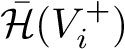 defined in (2.5), together with the transition intensities governing this process, the observed data likelihood can be formulated assuming biospecimens collected at all visits are assayed. The corresponding observed data likelihood contribution for the marker-failure process is then given by
\[\begin{aligned}{}{\prod \limits_{i=1}^{n}}\Bigg\{& {\prod \limits_{j=2}^{{A_{i}}({V_{i}})}}P({Z_{i}}({a_{ij}})\mid {Z_{i}}({a_{i,j-1}}),{X_{i2}})\\ {} & \times {\sum \limits_{k=0}^{1}}\Big\{P\left({Z_{i}}({V_{i}^{-}})=k\mid {Z_{i}}({a_{i{A_{i}}({V_{i}})}}),{X_{i2}}\right)\\ {} & \hspace{2em}\hspace{1em}\hspace{2.5pt}\times {\lambda _{2}}{({V_{i}}\mid {X_{i1}}({V_{i}^{-}})=k,{X_{i2}})^{{\delta _{i}}}}\Big\}\Bigg\}\hspace{0.1667em}.\end{aligned}\]
However, such complete assessment may be prohibitively expensive in many studies. We therefore seek cost-effective sampling strategies that retain the key advantages of this joint modeling framework while remaining feasible under realistic assay constraints. Specifically, we propose a sub-sampling scheme in which some individuals are selected for complete longitudinal assessment of their biospecimens over visits, and some are selected for a single assessment of the baseline (first-visit) biospecimen value. The rationale for this strategy is that individuals selected for complete longitudinal assessment of their samples enable estimation of the marker transition intensities, which in turn facilitates suitable use of data from those for whom only a single biospecimen is assayed. There are, however, individuals who experience events that are not sub-sampled in this scheme so there is the potential for some loss of information.
Suppose we have n individual processes, each with ${m_{i}}\ge 1$ clinical visits by the administrative censoring time for individual i, $i=1,\dots ,n$. For all individuals, biospecimens are sampled and stored at each clinic visit, yielding a total of ${m_{\cdot }}={\textstyle\sum _{i=1}^{n}}{m_{i}}$ biospecimen samples across all n individuals. Suppose that instead of assaying all ${m_{\cdot }}$ biospecimens, budgetary constraints permit only an average of ${\mu _{b}}$ assays (${\mu _{b}}\lt {m_{\cdot }}$) across these individuals. In Section 3, we investigated strategies allocating only one assay per individual. We let ${n_{L}}$ represent the number of individuals for whom all biospecimens are assayed and let ${n_{S}}$ be the number of individuals from the remainder of the cohort for whom the first available biospecimen will be assayed. Let ${R_{iL}}$ indicate individual i is selected to be followed longitudinally for complete assays of biospecimens over time, ${R_{iS}}$ indicate the individual is selected for a single assay of the biospecimen collected at the first visit, $i=1,\dots ,n$, then ${n_{L}}={\textstyle\sum _{i=1}^{n}}{R_{iL}}$ and ${n_{S}}={\textstyle\sum _{i=1}^{n}}{R_{iS}}$. Note under this selection strategy, an individual is either selected to be in the longitudinal subsample (${R_{iL}}=1,{R_{iS}}=0$), selected to be in the single-measurement subsample (${R_{iL}}=0,{R_{iS}}=1$), or not selected at all (${R_{iL}}=0,{R_{iS}}=0$). Let
denote the total number of assays conducted among those in the longitudinal subsample, we have the total number of assays ${m_{b}}={m_{L}}+{n_{S}}$ with $E({m_{b}})={\mu _{b}}$ to satisfy the budget constraint. A question then naturally arises: how should we allocate ${m_{b}}$ assays between the longitudinal and single-measurement subsamples? In other words, what fraction of ${m_{b}}$ should be allocated to ${m_{L}}$?
We consider independent random sampling, where the probability of being selected into the longitudinal subsample is $P({R_{iL}}=1,{R_{iS}}=0)={\pi _{L}}$, the probability of being selected into the single-measurement sample is $P({R_{iL}}=0,{R_{iS}}=1)={\pi _{S}}$, and the probability of not being selected into either sample is $P({R_{iL}}=0,{R_{iS}}=0)=1-{\pi _{L}}-{\pi _{S}}$, with ${\pi _{L}}+{\pi _{S}}\lt 1$. Selection into both subsamples is not allowed, so $P({R_{iL}}=1,{R_{iS}}=1)=0$. Moreover, we have $P({R_{iL}}=1)={\pi _{L}}$ and $P({R_{iS}}=1)={\pi _{S}}$. Under this framework and sampling scheme, the observed data likelihood contribution from one individual for the marker-failure process can be written as
\[ {L_{i}}\propto {\left\{{\pi _{L}}{L_{iL}}\right\}^{{R_{iL}}}}\hspace{0.1667em}{\left\{{\pi _{S}}{L_{iS}}\right\}^{{R_{iS}}}}\hspace{0.1667em}\]
where ${L_{iL}}$, ${L_{iS}}$ denote the contributions from the longitudinal and single-measurement subsamples respectively, with explicit forms
\[\begin{aligned}{}{L_{iL}}\propto & {\prod \limits_{j=2}^{{m_{i}}}}P\left({Z_{i}}({a_{ij}})\mid {Z_{i}}({a_{i,j-1}}),{X_{i2}}\right)\\ {} \hspace{2.5pt}& \times {\sum \limits_{k=0}^{1}}\Big\{P\left({Z_{i}}({V_{i}^{-}})=k\mid {Z_{i}}({a_{i,{m_{i}}}}),{X_{i2}}\right)\\ {} & \hspace{2em}\hspace{1em}\hspace{2.5pt}\times {\lambda _{2}}{({V_{i}}\mid {X_{i1}}({V_{i}^{-}})=k,{X_{i2}})^{{\delta _{i}}}}\Big\}\end{aligned}\]
and
\[\begin{aligned}{}{L_{iS}}\propto {\sum \limits_{k=0}^{1}}\Big\{& P\left({Z_{i}}({V_{i}^{-}})=k\mid {Z_{i}}({a_{i1}}),{X_{i2}}\right)\\ {} & \times {\lambda _{2}}{({V_{i}}\mid {X_{i1}}({V_{i}^{-}})=k,{X_{i2}})^{{\delta _{i}}}}\Big\}\end{aligned}\]
where ${V_{i}}=\min ({T_{i}},{C_{i}})$ and ${\delta _{i}}=1({V_{i}}={T_{i}})$. With a sample of n independent individual processes, the overall observed data likelihood is then $L(\theta )={\textstyle\prod _{i=1}^{n}}{L_{i}}(\theta )$ where $\theta ={({\theta ^{\prime }_{0}},{\theta ^{\prime }_{1}},{\theta ^{\prime }_{2}})^{\prime }}$ denotes parameters associated with the marker-failure process defined in (3.11a) and (3.11b). A maximum likelihood estimator $\hat{\theta }$ can then be obtained by maximizing the observed data likelihood. The Fisher information $\mathcal{I}(\theta )=E\left\{-\partial \log {L_{i}}(\theta )/\partial \theta \partial {\theta ^{\prime }}\right\}$ can be written as a weighted sum of the Fisher information contributed from the longitudinal and single-measurement subsamples
\[ \mathcal{I}(\theta )={\pi _{L}}{\mathcal{I}_{L}}(\theta )+{\pi _{S}}{\mathcal{I}_{S}}(\theta )\hspace{0.1667em},\]
where
\[ {\mathcal{I}_{L}}(\theta )=E\left\{-\partial \log {L_{iL}}(\theta )/\partial \theta \partial {\theta ^{\prime }}\right\}\]
and
\[ {\mathcal{I}_{S}}(\theta )=E\left\{-\partial \log {L_{iS}}(\theta )/\partial \theta \partial {\theta ^{\prime }}\right\}\hspace{0.1667em}.\]
The asymptotic covariance matrix of $\hat{\theta }$ is given by ${\mathcal{I}^{-1}}(\theta )$. To identify an optimal sampling design under the assay budget constraint, we study the asymptotic variance of the regression coefficient estimators. Since $\mathcal{I}(\theta )$ depends on the sampling probabilities ${\pi _{L}}$ and ${\pi _{S}}$, the optimal design is determined by the specification of ${\pi _{L}}$ and ${\pi _{S}}$ under the budget constraint.To characterize this constraint, we next relate the sampling probabilities ${\pi _{L}}$ and ${\pi _{S}}$ to the assay budget. Taking the expectation of ${m_{b}}={m_{L}}+{n_{S}}$ on both sides gives
where
and
with $\bar{\mu }=E({m_{i}})=E\{{A_{i}}(\tau )\mid {A_{i}}(\tau )\ge 1\}$ denoting the expected number of visits (and thus biospecimens) per individual by the administrative censoring time conditioning on having at least one visit. We can thus re-write (4.1) as
With pre-specified values of ${\mu _{b}}/n$ and $\bar{\mu }$, the budget constraint in (4.2) implies that ${\pi _{S}}$ is uniquely determined by ${\pi _{L}}$. Consequently, the Fisher information $\mathcal{I}(\theta )$ and corresponding asymptotic variance of the regression coefficient estimators can both be expressed as functions of ${\pi _{L}}$ alone. This allows us to identify the optimal value of ${\pi _{L}}$ that minimizes the asymptotic variance under the specified assay budget.
For practical interpretation, we re-parameterize this allocation strategy in terms of
which represents the fraction of total assays allocated to the longitudinal subsample. We next investigate the asymptotic variance of $\hat{\beta }$ as a function of ${\phi _{L}}$. We follow the model specifications and parameter settings of Section 3.3 and let the failure rate be ${\pi _{2}}=0.1,0.25,0.5$, or 0.8. We set ${\mu _{b}}/n=0.5$ or 1 and $\bar{\mu }=4$ or 8. For each value of ${\phi _{L}}$, we compute the asymptotic relative efficiency of $\hat{\beta }$, defined as
\[ \text{ARE}(\hat{\beta })=\frac{\text{asvar}(\hat{\beta })}{{\min _{{\phi _{L}}}}\text{asvar}(\hat{\beta })},\]
and plot $\text{ARE}(\hat{\beta })$ against ${\phi _{L}}$ in Figure 6. The optimal values of ${\phi _{L}}$ vary between 5% to 25% and the corresponding asymptotic variances of $\hat{\beta }$ are provided in the legends of the plots. Across all parameter settings, there is a common pattern: the asymptotic relative efficiency of β increases rapidly and then gradually decreases when the fraction of ${m_{L}}$ increases from 0 to 1. This is because when ${\phi _{L}}$ is very small, we have more individuals with fewer repeated measurements of the marker value so that we lose information about the marker transitions; when ${\phi _{L}}$ is larger, on the other hand, we have fewer individuals with more repeated marker measurements, so we lose information on the failure time. Comparing various levels of failure rate ${\pi _{2}}$, the optimal fraction ${\phi _{L}}$ is larger with higher ${\pi _{2}}$; additionally, the rate of change in the relative efficiency is also larger. The asymptotic variances are overall smaller when we have more budget on the number of assays (${\mu _{b}}/n=0.5$ vs ${\mu _{b}}/n=1$). Although these numerical results are based on specific simulation settings, the proposed design framework is general: for any given study setting and assay budget, investigators can vary ${\phi _{L}}$ over its feasible range, evaluate the corresponding asymptotic variance, and identify the value that minimizes asymptotic variance to determine the corresponding sub-sampling design.Figure 6
Asymptotic relative efficiency of ${\hat{\beta }_{1}}$ (left panel) and ${\hat{\beta }_{2}}$ as a function of ${\phi _{L}}$ for ${\pi _{2}}=0.1,0.25,0.5,0.8$, ${\mu _{b}}/n=0.5,1$ and $\bar{\mu }=4,8$; the asymptotic variances are obtained from the expected information matrix $\mathcal{I}(\theta )$ with the expectation carried out by Monte-Carlo integration with 500,000 replications.
5 Arthritis Mutilans in PsA
An illustrative example of the proposed selection strategy is given here by applying the method to data from the University of Toronto Psoriatic Arthritis Cohort Study. Psoriatic arthritis (PsA) is a complex rheumatic disease defined as a chronic inflammatory arthritis associated with psoriasis. The University of Toronto PsA Clinic at the Centre for Prognosis Studies in The Rheumatic Diseases at Toronto Western Hospital maintains a comprehensive database of patients diagnosed with PsA [10]. Individuals with a prior diagnosis of PsA are recruited to participate in the cohort and are followed prospectively over time to monitor the severity of disease progression. C-reactive protein (CRP) is a substance produced by the liver in response to inflammation, and a CRP blood test measures its level to detect inflammation from acute conditions or to monitor the severity of disease in chronic conditions. Erythrocyte sedimentation rate (ESR) is another blood test used to detect inflammation in the body. While similar to CRP in its purpose, ESR measures different aspects and can sometimes be used together with CRP for a more comprehensive view of inflammation. Both CRP and ESR measurements can only be taken during periodic clinical visits through blood tests. The primary interest here lies in studying the effect of the time-dependent covariate denoted ESR_CRP (which indicates if either ESR or CRP is elevated) on the time to the development of five or more damaged joints in patients with PsA. This represents a sufficient degree of damage that it satisfies the condition for a severe form of arthritis called arthritis mutilans [11].
We focus on a total of $n=1123$ patients with a prior diagnosis of PsA who had made at least one follow-up visit after recruitment into the study. For each individual, the reported age at PsA diagnosis is taken as the time origin. At each subsequent clinical visit, data including the ESR and CRP results from the blood tests, the date of the blood test, and the number of cumulative damaged joints were recorded. The age of onset of PsA varies from 4 to 49 years (with an average of 39.07 and S.D. of 13.57) across patients in this cohort, and the number of visits made per individual during their follow-up period ranges from 1 to 62 (with an average of $\bar{\mu }=9.98$ and S.D. of 12.42). Additionally, 274 (24.4 %) patients were observed to develop five or more damaged joints.
Instead of using all ${m_{\cdot }}=11204$ measurements of the ESR_CRP marker value, we imagine that the measurements were not available and consider a budgetary constraint. We subsample the visit times at which samples are available by our proposed cost-effective sampling strategy for a joint analysis of the ESR_CRP marker and the development of arthritis mutilans. We consider a fixed covariate of HLA-B27 and consider budgets ${\mu _{b}}$ to be $0.5n$, n or $2n$. With a pre-specified value of ${\phi _{L}}$ (i.e., the fraction of the marker measurements in the longitudinal subsample to the total budget), ${\pi _{L}}$ and ${\pi _{S}}$ can be determined via (4.2) and (4.3). We then select a subsample of marker measurements accordingly for the joint analysis. Our goal is to empirically investigate the variance of the coefficients of both ESR_CRP and HLA-B27 covariates under different specifications of ${\phi _{L}}$. When ${\mu _{b}}=0.5n$ or n, we choose ${\phi _{L}}=0.2,0.4,0.6$, or 0.8; when ${\mu _{b}}=2n$, we choose ${\phi _{L}}=0.6,0.7,0.8$, or 0.9, since we have to assign at least half of the budget to the longitudinal subsample (i.e., ${\phi _{L}}\gt 0.5$) to ensure ${\pi _{S}}\lt 1$. Time-homogeneous transition intensities are fitted for the joint multistate model, and the results of the estimates of the regression coefficients under various specifications of ${\mu _{b}}$ and ${\phi _{L}}$ are summarized in Table 1. For ${\mu _{b}}=0.5n$ or n, a minimum variance of the effect of the time-dependent marker ESR_CRP on failure is achieved when we assign 40% of the measurement budget to the longitudinal subsample, while a minimum variance of the effect of the fixed covariate HLA-B27 is achieved at 60%. For ${\mu _{b}}=2n$, the minimum variance of both the marker effect and the fixed covariate effect is achieved when ${\phi _{L}}=60\% $. Additionally, the estimated variance of both effects decreases as we have more measurement budget (data) for the time-dependent ESR_CRP value. The point estimates of the ESR_CRP effect are comparable when ${\phi _{L}}\lt 0.6$ but not when ${\phi _{L}}\gt 0.6$. This may be due to the small censoring rate of the original data, meaning that selecting fewer individuals (and thus having more longitudinal marker measurements) results in less data on observed failures.
Table 1
Joint analyses of the ESR_CRP and failure processes with a fixed covariate of HLA-B27 using subsamples selected under different specifications of ${\mu _{b}}$ and ${\phi _{L}}$; time-homogeneous baseline transition intensities are fitted; variance estimates are obtained through observed information matrix averaged over 500 repetitions.
| Covariate | |||||
| ESR_CRP (${\beta _{1}}$) | HLA-B27 (${\beta _{2}}$) | ||||
| ${\mu _{b}}/n$ | ${\phi _{L}}$ | EST | VAR | EST | VAR |
| 0.5 | 0.2 | 1.639 | 2.848 | 0.175 | 0.590 |
| 0.4 | 1.464 | 2.449 | 0.293 | 0.588 | |
| 0.6 | 1.361 | 2.608 | 0.225 | 0.532 | |
| 0.8 | 0.941 | 2.634 | 0.291 | 0.574 | |
| 1 | 0.2 | 1.660 | 1.343 | 0.231 | 0.417 |
| 0.4 | 1.522 | 1.288 | 0.270 | 0.339 | |
| 0.6 | 1.355 | 1.305 | 0.285 | 0.312 | |
| 0.8 | 0.917 | 1.324 | 0.258 | 0.351 | |
| 2 | 0.6 | 1.229 | 0.705 | 0.283 | 0.200 |
| 0.7 | 1.134 | 0.732 | 0.270 | 0.211 | |
| 0.8 | 0.974 | 0.974 | 0.268 | 0.231 | |
| 0.9 | 0.798 | 0.791 | 0.263 | 0.273 | |
6 Discussion
The bias in Cox regression coefficients arising from the carry-forward approach has recently been studied formally [7, 12]. To address this issue, joint modeling of continuous marker processes and failure times is needed, with most models for the marker trajectory having an additive form with subject-specific random effects accommodating heterogeneity in the marker paths and a serial dependence. The association between the marker process and the failure process is accommodated by incorporating shared or correlated random effects to the failure time model [15, 20]. Conditioning on the random effects, the failure time process and the marker processes are typically assumed to be independent, but a joint model can be obtained by integrating over the random effects. Such joint models often require a strong assumption about the distributions of the marker processes [3, 21] and are less appealing when the failure event is death, as the marker process does not terminate upon death [19]. Other strategies for dealing with intermittent observation of marker processes do not involve joint modeling. de Bruijne et al. [9] proposed a way of attenuating the bias using a weighted Cox regression method where weights decay as a function of time from the most recent marker measurement; this reduces the bias by down-weighting contributions to the partial score function when it is a long time since the marker measurement. Other methods involving using smoothing techniques to impute the missing “current” marker values at failure times have been explored [16, 18, 2].
In medical research, it is common to discretize continuous biomarkers by specifying cut-points agreed upon by researchers; in some settings these may be thresholds delineating meaningfully different disease states. Such discretization can be appealing since it enables a joint multistate model of the marker and failure processes by specification of a discrete state spacing incorporating different levels of marker states and an absorbing state for the terminal effect of death [5]. Moreover, in settings where marker values are recorded at clinic visits or when an individual seeks medical care, the visit times are often associated with the values of the marker process. It is then crucial to account for such association between the clinical visit process and the disease process for valid inference of the marker effect as the observation process conveys information about the disease process [5, 6].
We studied the association between a time-dependent biomarker and a failure time of interest in settings where biomarker measurements are only available at intermittent clinical visits. We introduced a multistate model for the joint marker-failure process by discretizing the continuous biomarker into two levels. This model formulation allows for natural extensions to accommodate dependent observation processes [7], and can be generalized to accommodate more marker states and higher-dimensional discrete markers. Markov transition intensities with proportional hazard models were adopted to govern the disease dynamics. With marker values available at each clinical visit, a joint analysis can be conducted for the marker-failure process. We also considered budgetary constraints on assessing marker values at clinical visits and investigated the asymptotic bias of four commonly used but naive ad hoc strategies for statistical inference arising from misspecified Cox models. Our findings indicated that there is generally an attenuation of the estimated regression coefficients, particularly for the marker effect, even when the visit process is completely independent of the disease process. To address this, an alternative cost-effective strategy has been proposed to mitigate bias under budgetary constraints which involves efficient selections of individuals. The asymptotic relative efficiency of estimators obtained from this proposed strategy under different designs has been explored and an optimal one can thus be determined.
As we only have focused on simple random sampling for individual selection, a natural alternative to the selection strategy is to consider outcome-dependent sampling for individual selection to the two subsamples. Specifically, we might intentionally select all individuals with an observed failure and assess their marker values using all biospecimen samples. Besides selecting individuals with either a single assay or complete assays of biospecimens, we could also consider selecting several specific visits at which the collected biospecimen is assayed for each individual, and the visits selected could vary across individuals. In general, if we let ${R_{ij}}=1$, $j=1,\dots ,{m_{i}}$, indicate the biospecimen collected at the jth visit for individual i is assayed for a marker value, the budgetary constraint becomes ${m_{b}}={\textstyle\sum _{i=1}^{n}}{\textstyle\sum _{j=1}^{{m_{i}}}}{R_{ij}}$. Various models can be specified for the joint distribution of the selection indicators ${R_{ij}}$, allowing for the formulation of a joint likelihood of the selection indicators and the marker-failure process. Fisher information can then be derived for determining an optimal design of the parameters related to the selection distributions.
The robustness of the multistate model for the joint marker-failure process can be improved by adopting piecewise constant baseline transition intensities. Random effects could be incorporated into the transition intensities to account for unexplained heterogeneity at the individual level. More complex multistate disease process can be considered when there is more than one clinical event of interest. Additionally, the multistate model can be extended to accommodate a higher-dimensional marker process via the use of more cut-points for the marker value or through the consideration of multiple time-dependent markers. Mixture multistate models might also be of interest when there is a portion of the population not susceptible to the event of interest. These models can separate the susceptible and non-susceptible subpopulations, providing more accurate estimates of the effects of covariates on the failure risk. This approach could be particularly useful in settings where heterogeneity in the population’s response to covariates or failure susceptibility is expected.