1 Introduction
Concerns of reproducibility and replicability are continually on the rise across many academic disciplines, with contributing factors including “p-hacking,” improper statistical analysis, and poor practices in data management and data sharing. In fact, the problem of p-hacking has become so widespread that, in 2016, the American Statistical Association felt it necessary to release a statement on p-hacking, the proper usage of p-values, and the impact of misusing p-values on reproducibility [19], and a psychology journal actually banned the usage of p-values entirely [20]. Problems with data sharing and data availability have also generated concern; for example, starting in 2014, the journal PLOS ONE implemented policies to promote data sharing and encouraging researchers to make the data used in its publications publicly available [6]. The question of whether these policies are feasible and effective, especially due to confidentiality concerns, has sparked discussion. Nonetheless, some positive changes have been reported. For example, a study [7] done in 2023 finds that, for the journal Management Science, the “Data and Code Disclosure” policy implemented in 2019 marked a substantial increase in the proportion of articles that could be reproduced.
In this paper, we conduct analyses on both of these factors—p-hacking and lack of responsible data sharing—that contribute to the “reproducibility crisis”.
In consideration of the former problem, p-hacking, one goal of this paper is to examine a currently under-examined facet of this issue, which we will refer to as “reverse p-hacking.” The term “reverse p-hacking” has been used previously to describe “[ensuring] that tests produce a nonsignificant result” [4], which is similar in spirit to our intended meaning. We will use the same vocabulary, but our specific aims are to investigate the usage of “reverse p-hacking” in the process of model validation. We seek to examine the practice, intentional or otherwise, of using tests with low power to validate models, thus producing insignificant p-values that support the models based on which authors draw conclusions.
Here, we define our specific area of focus: we analyze published papers that develop a binary logistic regression model, then use the Hosmer-Lemeshow goodness-of-fit test to validate it. This particular topic is of interest due to the prevalence in usage of the Hosmer-Lemeshow test. The binary logistic regression remains one of the most popular statistical models in application, and goodness-of-fit tests are typically performed to validate the final logistic regression models. When the data are grouped, the standard chi-square test or deviance test are asymptotically valid [5]; however, when one or more predictors are continuous, these tests cannot be used. The Hosmer-Lemeshow test [9] was developed to address this issue. It became and remains a very widely-used [12] goodness-of-fit test for logistic regression on ungrouped data and is widely cited (see our analysis on trends for citations, with data downloaded from the online article via Taylor & Francis), and it is also taught in popular textbooks (one of which was written by Hosmer & Lemeshow themselves [10] along with Rodney X. Sturdivant).
Recently, concerns have been raised regarding the use of the Hosmer-Lemeshow test for logistic regression (e.g. [13], [21]). One major concern is the test’s lack of power in detecting inadequacy of the model being assessed, which can be especially serious when the model has missed important variables available in the data that should have been included (i.e. they significantly improve the model when included). If these theoretical concerns are practically relevant, the usage of the Hosmer-Lemeshow test may lead to, if not intentional, passive “reverse p-hacking” for justification of a model by the data analyst.
One goal of this paper is therefore to investigate the ability, or lack thereof, of the Hosmer-Lemeshow test to detect a poorly-fit model. We conduct a practically-oriented examination of the test’s applications—specifically, its actual usage in published research.
In addition to the analysis on the Hosmer-Lemeshow goodness-of-fit test, we also investigate the second factor of the reproducibility problem highlighted above: the lack of proper data sharing practices, either by not sharing data at all or by supplying data that cannot be used to reproduce the results of the paper. Collecting our own data is outside the scope of this project, so we rely on raw data being made available by authors to reproduce results described in their papers. Therefore, since reproducing the results described in the papers is a necessary first step in our analysis of the Hosmer-Lemeshow test, we also examine potential problems with data availability. We investigate this problem from two different angles. First, whether data is made available, particularly when the authors claim that data already is or can be made available. Second, for the data provided—whether they are already included in a “Supplemental Materials” section of the paper or supplied by request—we check if they are actually usable to reproduce the results described in the paper.
When we say “reproducing results”, we specify two objectives: the first is to replicate the results of the regression itself, preferably exactly, by getting identical or very nearly identical odds ratios as those reported in the given paper; the second is to reproduce the conclusion of the Hosmer-Lemeshow test—simply obtaining a non-significant p-value at the threshold indicated in the paper, and therefore reaching the same conclusion as the paper’s, is sufficient for our purposes. It is after the successful replication of these two components of the paper’s results that we begin our analysis of the Hosmer-Lemeshow test itself.
2 Study Design
2.1 Search Term Engineering
To examine publications in a systematic way, we designed a search term set on Google Scholar, then reviewed the papers in the order that Google Scholar displayed them. To obtain the highest proportion of relevant and usable papers in our analysis, we used a specific set of keywords as the search terms in Google Scholar.
Naturally, to obtain papers that use the Hosmer-Lemeshow test, we include the term “hosmer-lemeshow.” During the process of search-term engineering, we found that raw data is rarely easily accessible, but the few papers that did have data available usually included a data availability statement. We thus extracted some of the most commonly used phrases in such data availability statements, such as “data availability,” “availability of data,” and “relevant data are available,” and included them in our search term set using the “OR” keyword. Using these search terms yielded a high proportion of desired results, but a large number of them included a calibration for the model. To avoid this complexity, we added an additional term -calibration NEAR hosmer-lemeshow.
Thus, the final search term set used to find papers on Google Scholar was: “hosmer-lemeshow” AND “data availability” OR “availability of data” OR “relevant data are available” -calibration NEAR hosmer-lemeshow.
2.2 Dataset Organization
We created our own dataset to keep a record of all papers we analyzed. We organize the dataset as follows: the first column is the title of the paper, the next is the year of publication, then the link Google Scholar provided, then the “availability statement status” of the paper—whether the paper included data availability statement or not. There are 6 categories for the “statement status:”
The last column indicates the paper’s replication status: whether we ultimately were able to replicate the published logistic regression (matching odds ratios as reported in the paper), or if there were roadblocks, such as missing variables.
-
1. “Not Relevant”: These papers are not usable for our analysis, e.g. Hosmer and Lemeshow’s own paper, or some kind of meta-analysis done on previous results.
-
2. “No Statement”: These papers had no data availability statement. These papers reference the availability of data obtained from other sources that they needed to produce their own results, not whether they will provide their raw data to their readers.
-
3. “Contacted”: In these cases, the statement directs the reader to email the corresponding author(s). It is stated that data are available upon reasonable request.
-
4. “Claimed Available”: In these cases, the data availability statement reads, approximately, “relevant data are included in the paper or the Supporting Materials section,” but the data is actually not accessible, or the supplemental materials provided are not raw data.
-
5. “Claimed Not Available”: This means that the statement is present, but it directly informs the reader that data cannot be made available, usually due to confidentiality concerns regarding sensitive data.
-
6. “Data Available”: This means that raw data is included, usually in the “Supporting Information” section of the paper.
2.3 Timeline of Research
Systematic review of the papers using the search term set described above began in August of 2022.
As of the date 23 August, 2023, all papers in the first 8 pages of results in Google Scholar are included in our dataset of analyzed articles in the order they appeared in. However, because the order of results in Google Scholar shifts over time, there are articles included at the bottom of our dataset (specifically, the last 8) that occur on later pages of a Google Scholar Search. These papers were examined at earlier dates and are now not displayed within the first 8 pages of Google Scholar. We include them in our dataset for the sake of completeness. Therefore, we have 88 examined papers in total.
We briefly note that, due to the inclusion of the three search terms about data availability, these 88 papers are, in the far majority, published within the last few years, with 74% published 2020 or later, and 87.5% published 2016 or later. The Google Scholar search results with these search terms omitted are far older.
3 Results
3.1 Data Availability of Examined Publications
Out of 88 papers, we deemed 81 relevant to our research, so we will examine the data availability claims and the final outcomes (whether data was actually obtainable and ultimately usable) of these 81 papers.
Even when a data availability statement was present, some were merely suggestions to contact the corresponding author(s), and even when data are claimed to be available, what was provided was not always raw data or usable data.
We therefore present a detailed breakdown of the 81 papers in question and their data availability: in Figure 1, we visualize the set of papers in a tree, where each set of branches divides its node into subsets using some data availability status criterion. For example, the first set of branches divides the root node into two categories: one for papers that have data availability statements, and one for papers that do not. For each child node, the percentage of its parent node its category encompasses is labeled.
After omitting irrelevant papers (e.g. Hosmer and Lemeshow’s own paper) and papers with no data availability statement, we discard 24 papers and retain 64. We describe the breakdown of the data availability statement categories, i.e. claiming “data is available” or “data is not available,” or including a comment to “contact the author(s),” and the ultimate true availability of the data (i.e. whether raw, usable data can actually be obtained).
Out of the 64 papers with data availability statements, 43 claimed data would be made available upon reasonable request, 15 claimed data to be available in the paper or its “Supporting Information” section, and 6 claimed confidentiality concerns. 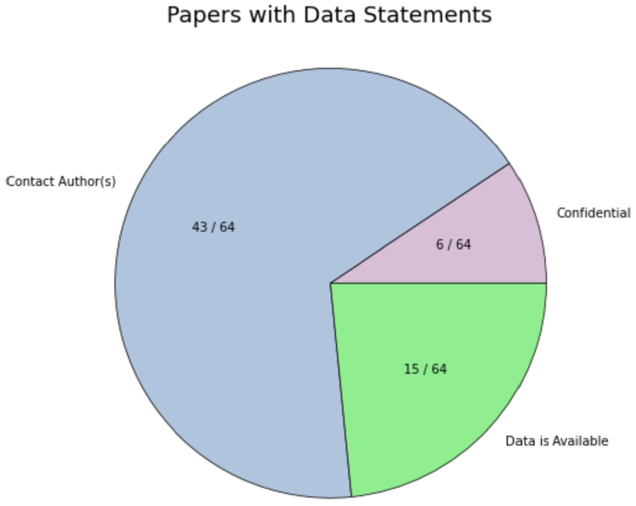
We further examine the former two categories: out of the 15 papers that claimed data are available, 4 papers included supplemental materials that were not raw data, 2 papers had links to data that are not functional, 4 provided data that are not usable due to missing predictors or the outcome, and 5 provided usable raw data. 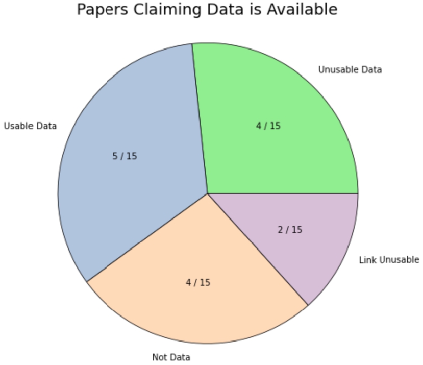
Out of the 43 papers for which we contacted corresponding author(s), 33 yielded no response (the most recent email sent was on 23 August, 2023), 7 responses cited confidentiality concerns, some requesting certification with institutions in their home country (which we did not pursue), and some requesting specific publication details (which we were not able to provide). We encountered 1 message send error, in which the email was not delivered, possibly due to an invalid or outdated email address. In 2 cases, usable raw data was provided by email. 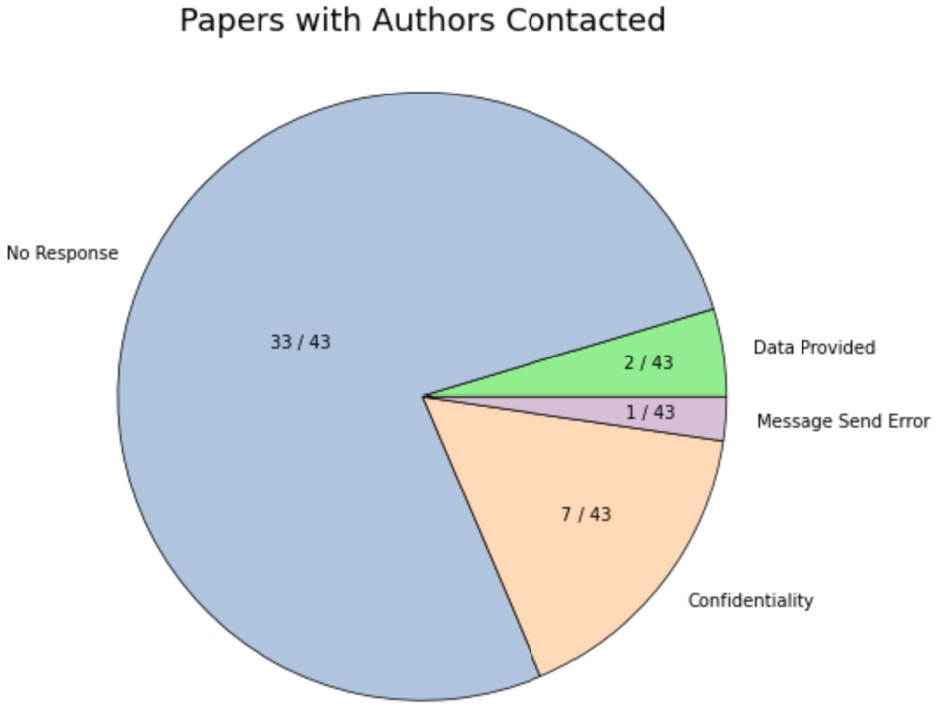
Thus, in total, we find several concerning trends in published research regarding data availability:
Even though a majority of papers claim that data already is or can be made available, for very few papers were we actually able to obtain usable data. This finding offers some support of earlier research concluding that mandating these data availability statements does not make data sharing substantially more effective [16].
-
1. Lack of data availability statement: Unless the presence of a data availability statement is explicitly included in our set of search terms, published papers displayed in a Google Scholar search often do not include one.
-
2. Providing non-data: Data are claimed to be available, but the supporting materials were actually summary statistics or other materials, not raw data used to build the regression model.
-
3. Providing incomplete data: Data given has variables omitted without disclaimer or otherwise clear indication of reason for its omission. Processes were sometimes described for the derivation of variables ultimately used in the regression, but not in enough detail to allow reproduction of results.
-
4. Ignoring email requests: Although the data availability statement welcomes requests sent by email to the corresponding author(s), more than 70% of emails received no response.
3.2 Data Description for Papers Included in Further Analysis
There are 7 papers included in the ultimate analysis on the reliability of the usage of the Hosmer-Lemeshow test, and because two papers developed 2 separate logistic regression models, there are a total of 9 models analyzed.
The first step is replicate the authors’ selected models as closely as possible, as a baseline for comparison. To do this, we analyze the available datasets.
3.2.1 Dataset Summary
We summarize the basic metadata of each dataset we used to replicate the models.
We note in Table 1 the number of observations (rows) in the dataset, excluding null rows, the number of total variables (columns) included in the dataset by the authors, and the number of variables ultimately included in the final multivariate binary logistic regression model, including the outcome variable.
Table 1
Paper Datasets Basic Metadata.
| Paper Authors | Number of Observations | Total Variables | Variables in Model |
| Mithra et al. [14] | 450 | 222 | 7 |
| Gebeyehu et al. [8] | 421 | 53 | 2 |
| Campos et al. [3] | 198 | 37 | 3 |
| Peterer et al. (Model 1) [15] | 311 | 66 | 6 |
| Peterer et al. (Model 2) [15] | 311 | 66 | 6 |
| Zhu et al. (Model 1) [22] | 76,359 | 23 | 3 |
| Zhu et al. (Model 2) [22] | 77,018 | 26 | 7 |
| Kibi et al. [11] | 5,313 | 37 | 7 |
| Wang et al. [18] | 115 | 6 | 5 |
3.2.2 Datasets Enabling Exact Replication of Expected Results
Five of the analyzed models, with two from the same paper, had data exactly as described. In most cases, other variables that were not included in the final multiple regression model were also present, either because they were included in univariate analyses, because the authors deemed them otherwise important to keep in the dataset, or they were not removed for the sake of completeness. To replicate the authors’ models exactly, we first removed these extraneous variables during this step, keeping only those specified to be in the final multivariate model.
For categorical variables, it was necessary to map them to binary or otherwise numeric values (one-hot encoding). When the binary logistic regression was run, the odds ratios were identical or nearly identical to the described results in the paper (it was sometimes necessary to use the additive reciprocal of the output coefficient to match the given odds ratios, when the coefficients produced by the regression were the opposites of those reported).
3.2.3 Datasets with Anomalies in the Replication Process
For three of the models, there were anomalies in the data, omissions in the description of the data, or other roadblocks in replicating the papers’ reported results exactly. We describe these three datasets here.
For the paper by Gebeyehu et al., only a subset of the data were made publicly available. The rest of the data were not released due to a data sharing policy (as relayed to us via an email conversation). We thus proceeded with the publicly available subset of the data, which includes 421 rows, and we attempted to replicate the results in the paper. Our odds ratios obtained are quite similar to those reported in the paper, and using Hosmer-Lemeshow obtains a non-significant p-value of nearly 1. The paper does not report an exact p-value, just stating that the significance level is 0.05 and that the p-value obtained was not significant.
For the paper by Kibi et al., the process of dealing with third-category responses to binary questions (such as “I don’t know whether I received a flu vaccine”) was not described. Experimenting with different methods of dealing with these third-category responses, we were still able to get extremely similar odds ratios/coefficients to those reported in the paper for all but one variable. However, we encountered another unexpected problem: when using the Hosmer-Lemeshow test, we obtain a significant p-value (with number of bins ranging from 2 to 15 tested) at the alpha = 0.05 level. The paper’s authors reported using a 0.05 significance level but did not report their exact p-value, and we did not receive a response to our email inquiring about the significant results.
For the paper by Peterer et al., there are two models built, each with the same set of predictors but a different outcome. One of the used variables in the two final multivariate logistic regressions, “Gender”, was not available due to confidentiality. However, the authors did not find this variable to be significant in either model. We thus attempted to run logistic regressions using the other variables, omitting the missing “Gender” variable. We find that our coefficients are quite close to those reported in the paper, despite the Gender variable being excluded. Upon using Hosmer-Lemeshow, we also find an insignificant p-value. We thus still choose to include this paper in the next stage of our analysis.
3.3 Reproducing Binary Logistic Regressions
For all 9 models, we obtained odds ratio values that are reasonably close to those reported by the authors. Nearly all were comfortably within the confidence interval reported in the results (far closer to the exact value reported than the boundaries). The one exception was a single predictor in the paper by Kibi et al., which was outside the reported confidence interval.
The p-values we obtained from conducting the Hosmer-Lemeshow test do differ from the ones reported in the papers. This is likely due to varying implementations of the Hosmer-Lemeshow test. Additionally, the number of bins used was not specified in any of the papers, so we used a default of 10 in the following reported values. An examination of the differing p-values resultant from bin count variation is included in later analysis in this paper. Despite the differences in p-values, the conclusions drawn, using a threshold $\alpha =0.05$, are consistent with those of the authors (with the exception described above for Kibi et al.).
We report our obtained p-values using the default bin number of 10, compared to those given in the original papers, in Table 2.
Table 2
Comparison of p-Values.
| Paper Title | Given p-Value | Obtained p-Value |
| Mithra et al. | Not Reported (> 0.05) | 0.299 |
| Gebeyehu et al. | Not Reported (> 0.05) | 1.0 |
| Campos et al. | 0.684 | 0.442 |
| Peterer et al. | 0.11 | 0.600 |
| Peterer et al. | 0.88 | 0.640 |
| Zhu et al. | 0.130 | 0.970 |
| Zhu et al. | 0.638 | 0.843 |
| Kibi et al. | Not Reported | 7.20e-10 |
| Wang et al. | 0.962 | 0.462 |
3.4 Hosmer-Lemeshow Sensitivity to Bin Count
To analyze the sensitivity of the Hosmer-Lemeshow test to the number of bins used in the implementation, we vary the bin count when conducting the test with the models we obtained. Existing concerns about the Hosmer-Lemeshow test include bin sensitivity: In a blog post by Paul Allison in Statistical Horizons [2], it was found that changing the bins from 8 to 9 changes the result from significant ($p=0.0499$) to not significant ($p=0.11$), and further increasing the bins to 11 increases the p-value to 0.64. To analyze these concerns on our collection of datasets, we use bins 5–16, and examine the resultant p-value.
We find that varying the bin count does not change the conclusion for any of the models. In 8 out of 9 models, the p-value is above the reported cutoff threshold, 0.05, for all 12 bin counts. For the 1 model in which we obtained a significant p-value with the default 10 bins, the p-values are significant for all 12 bins.
We do notice, however, that there is a rather large range the p-values take depending on the bin count. Many papers have a range as wide as 0.6 (excluding the paper with a significant p-value, which had a range of several factors of 10), and in the paper by Mithra et al., the p-value dropped to 0.07, near the 0.05 threshold, with 8 bins.
3.5 Assessing the Efficacy of Hosmer-Lemeshow
We now study the efficacy of the Hosmer-Lemeshow test. We are interested in analyzing whether the Hosmer-Lemeshow goodness-of-fit test is able to detect a poorly-fit or non-ideal model. A comparison to the full model with all available predictors, the saturated model, is a requirement of a goodness-of-fit test for binary logistic regressions [10], so if, when we use additional predictors from the dataset, the model is significantly improved, this suggests that the Hosmer-Lemeshow test was not able to detect that the original model is not a proper fit—that the original model was missing information that can substantially improve model performance.
To test this, we consider not only those predictors ultimately chosen in the authors’ final multivariate logistic regression model, but also those predictors not selected (but still present in the data, of course). We work to produce an alternative model to the authors’ reported final model, and specifically, we require our model have a superset of the original predictors. The following describes the process in producing this alternative model:
Prior to discussing the comparison between the original and alternative models, we discuss the execution of the above process for each paper.
-
1. We begin with all available data. We first omit variables with too many null values. We also omit variables where the values are too complex (for example, if the value is description based, not numerical or categorical). We then omit variables that were either used in any way to construct the outcome, or are too similar to the outcome, such as a continuous version of the binary outcome variable.
-
2. To consider predictors that were not used in the authors’ final multivariate logistic regression, it was necessary to omit rows in which there were null values in the originally unused columns. This was done to ensure consistency in the regression comparison, and particularly in the comparison of the degrees of freedom. In certain cases, this caused fluctuations in how well the original model was able to be reproduced, but changes in odds ratios were not significant.
-
3. Using this dataset containing all acceptable predictors, we first re-run the original model proposed by the authors as a baseline. Next, using all predictors, we implement a backward stepwise regression to select the “ideal” subset of them (as defined by the backward stepwise regression process).
-
4. We then compare this model ultimately chosen in the backward stepwise regression with the original model chosen by the authors. We take note of the differences in predictors selected, then run a regression with the following set of predictors: We thus produce an alternative model, one with a superset of the original predictors.
First, we find that for two papers, Wang et al. and Mithra et al., the remaining predictors included in the data are difficult to extract due to missingness, encoding difficulties, or other factors (for example, convergence issues when there are too many binary variables included in the model). We thus do not include them in this section of analysis.
The paper by Gebeyehu et al., uses the Hosmer-Lemeshow test for variable selection rather than for validating their final multivariate regression, so we choose to analyze separately, and thus do not include it in this section of analysis.
We will thus focus on examining the remaining four papers using the methodology described above. For papers Campos et al. and the model for male patients in Zhu et al., we identified 3 and 4 additional variables that improve the model, respectively. For the model for female patients in Zhu et al., the backward stepwise regression process produced a subset of the original variables chosen by the authors, so we do not investigate this model further.
In the other cases, an alternative model was produced, but with deviations in the process described above, and a more detailed description of the methodology of constructing the model is required:
-
1. In the paper by Kibi et al., there is a column containing the age category of the participants, in which there are 5 categories. In the final regression model described in the paper, there is one binary age variable used, where the age categories are combined to form two categories: under 18 and over 18. We find that using the original “age category” variable instead of the binary “adult” variable yields a significantly better model.Another set of variables identified by the backward stepwise regression are the “education” variables, with 7 categories in total.We therefore examine three different alternative models: one with the binary age variable changed to 5 categories, one keeping the original binary age variable and adding the “education” variables, and one doing both.
-
2. In the paper by Peterer et al., the backward stepwise regression did not yield a significantly better model. However, we consider the encoding of a variable the authors did use: the Injury Severity Score (ISS) is a score ranging from 0–75. The column of raw ISS values are mapped to ISS groups, following the standard of a cutoff at 16: scores 9–15 are considered moderate, and 16 and above are considered severe. Some literature supports usage of an additional category: separating values above 16 into 16–24 and 25 and above [17]. We experiment with using the raw ISS score, a continuous variable, and using the ISS score with three categories instead of two. In both cases, we see an improvement in the model. We also note that when changing the discrete binary “ISS group” variable into the continuous version, there is no loss in degrees of freedom, but when we use the alternative discrete “ISS group” value, we lose 1 degree of freedom due to the addition of the third category. This consideration is naturally only relevant if dividing the score into a binary variable is not a rigid requirement.
We may use the Akaike information criterion (AIC) [1], a widely used model selection tool, to conduct a first comparison of the original and alternative models. We immediately see that the AIC scores of our alternative models are lower than those of the original models.
Next, we do a more rigorous comparison of the original versus the alternative models. We do this by examining the residual deviance. For two models where one has a subset of the predictors of the other, the larger model naturally has fewer degrees of freedom. Under the assumption that the smaller model is proper, the difference in the residual deviance follows a chi-square distribution with ${n_{2}}-{n_{1}}$ degrees of freedom, where ${n_{2}}$ and ${n_{1}}$ are the degrees of freedom for the larger and smaller models, respectively.
Table 3
AIC Scores.
| Paper Title | Original Model | Alternative Model |
| Campos et al. | 239.8 | 228.66 |
| Kibi et al. (with age) | 5520.3 | 5344.6 |
| Kibi et al. (with education) | 5520.3 | 5385.1 |
| Kibi et al. (with both) | 5520.3 | 5312.7 |
| Zhu et al. | 1471.1 | 1461.5 |
| Peterer et al. (continuous) | 266.98 | 211.45 |
| Peterer et al. (ternary) | 266.98 | 253.72 |
We thus may take the difference in the residual deviance, and use a chi-square test with the appropriate degrees of freedom to determine whether the discrepancy is significant.
We visualize our results in the Table 4, where the sub-rows are the residual deviance and degrees of freedom for the original and alternative models as well as the difference between them, which is the test statistic used. The last column is the p-value obtained using the chi-square distribution.
Table 4
Comparison of Original Model with Alternative.
| Paper Title | Original Model | Alternative Model | Test Statistic | p-Value |
| Campos et al. | 219.80 | 202.66 | 17.14 | 6.614e-4 |
| df = 188 | df = 185 | df = 3 | ||
| Kibi et al. (age) | 5498.3 | 5316.6 | 181.7 | 3.787e-39 |
| df = 5255 | df = 5252 | df = 3 | ||
| Kibi et al. (edu) | 5498.3 | 5353.1 | 145.2 | 1.403e-29 |
| df = 5255 | df = 5250 | df = 5 | ||
| Kibi et al. (both) | 5498.3 | 5274.7 | 223.6 | 6.680e-44 |
| df = 5255 | df = 5247 | df = 8 | ||
| Zhu et al. | 1463.1 | 1445.5 | 17.6 | 1.477e-3 |
| df = 76355 | df = 76351 | df = 4 | ||
| Peterer et al. (cont.) | 256.98 | 201.45 | 55.53 | n/a |
| df = 205 | df = 205 | n/a | ||
| Peterer et al. (ternary) | 256.98 | 241.72 | 15.26 | 9.368e-05 |
| df = 205 | df = 204 | df = 1 |
We thus find that the discrepancy in model performance is highly significant.
3.5.1 A Misuse of the Hosmer-Lemeshow Test
During our analysis of the usage of the Hosmer-Lemeshow test, we found that it was used incorrectly for a task unrelated to the nature of the test, i.e., the methodology of using the test for variable selection as described in Gebeyehu et al.
The authors did not use the Hosmer-Lemeshow test to analyze the goodness-of-fit of the final model, but was rather used it on each of the univariate regressions to test whether, for that predictor, the difference in expected and observed proportions is significant. The predictors that passed this test were then included in the further multivariate analysis.
We express skepticism about the validity of this methodology, and conduct the following two experiments:
These two experiments illustrate the fact that the Hosmer-Lemeshow test, by design, is not a proper tool for variable selection, and its usage in Gebeyehu et al. is therefore not suitable.
-
1. In this experiment, we generate y values randomly, and test whether the Hosmer-Lemeshow test allows predictors to pass the test despite having no predictive ability (the outcome being random).Ultimately, around 98% of runs, we obtain the result that all predictors have non-significant p-values, in fact, nearly all are almost exactly 1. As we can see from this experiment, the Hosmer-Lemeshow test is not capable of identifying when the variable is not very predictive—all predictors tested passed the test, despite the fact that the outcome values are randomly generated.
-
(a) Using a Bernoulli random value generator, we generate random outcome values with probability of success being 0.9, matching the proportion of positive outcomes in the actual data.
-
(b) We then use the Hosmer-Lemeshow test on a univariate logistic regression with each independent variable, and observe the p-values.
-
-
2. We conduct another experiment in the other direction: we consider whether the Hosmer-Lemeshow test would reject a significant predictor when conducting univariate analysis.In this experiment, we first randomly generate data in the following manner:We see that in this case, the Hosmer-Lemeshow test erroneously rejects an important predictor.
-
(a) Let variable ${x_{1}}$ be a value randomly generated from a uniform distribution with range [−5, 5].
-
(b) Let variable ${x_{2}}$ be equal to ${({x_{1}}+\epsilon )^{2}}$, where ϵ is noise randomly generated from a normal distribution with mean 0 and variance 2. Using this value for variance produces ${x_{1}}$ and ${x_{2}}$ vectors with a Pearson correlation coefficient of approximately 0.5.
-
(c) Let coefficients ${\beta _{1}}$ and ${\beta _{2}}$ both be 0.5, and let the intercept be ${\beta _{0}}=0$. We use these chosen values to calculate probabilities of being in the positive class for each row of data.
-
(d) Using Bernoulli random variables with the calculated probabilities for each row, we then generate values for each y.
-
(e) We now conduct two regressions: the first is a bivariate regression with both ${x_{1}}$ and ${x_{2}}$, and the second is a univariate regression with only ${x_{1}}$. For the bivariate regression, we check whether the coefficient for ${x_{1}}$ is significant, using a threshold of $\alpha =0.05$.
-
(f) We then use the Hosmer-Lemeshow test on the univariate regression with only ${x_{1}}$ and check whether the test rejects ${x_{1}}$ as a fit predictor for the outcome, mimicking the univariate analysis done in Gebeyehu et al. We find that, with approximately 95% of runs, although ${x_{1}}$ is deemed to be significant in the bivariate analysis, the Hosmer-Lemeshow test actually rejects the predictor.
-
4 Conclusion
The irreproducibility crisis is now widely recognized in the scientific community. There are a number of contributing factors, and two are addressed in this work; namely, the ability to obtain data and reproduce the same quantitative results by the same data analysis procedure, and the reliability of a statistical tool that is free from p-hacking or reverse p-hacking.
Our research has these two specific goals: to investigate the reproducibility of the results from published papers whose objective is to develop a logistic regression and validate their results using the Hosmer-Lemeshow test, and to investigate the adequacies of the widely-used Hosmer-Lemeshow test itself.
First, on the reproducibility of results in published research using authors’ data, we found serious discrepancies between data that are claimed to be available and data that are usable to reproduce results. Out of the 88 papers initially included in our study, 64 were relevant to our goals, and of these 64 papers that claim data are available or can be made available upon reasonable request, we were able to reproduce the results of only 7, an astonishingly small number. With most papers that have a data availability statement claiming that the raw data are available upon reasonable request, contacting the authors fails to receive a response. When data are claimed to be available in a supplemental materials section of the paper, the materials available are often not data. When raw data is indeed provided, the data is often unusable to reproduce the authors’ results, either due to missing variables or corrupted files.
Second, on the inadequacies of the Homser-Lemeshow goodness-of-fit test, we substantiated the theoretical concerns of its lack of power by demonstrating that the Homser-Lemeshow test failed to detect the improper models proposed by the authors in published research. In all 4 models that were ultimately tested, we were able to build a significantly better model, which we verified based on chi-square tests using the difference in residual deviance of our new proposed model and the authors’ original model. With such prevalence of the Hosmer-Lemeshow goodness-of-fit test in many fields of research, we demonstrated that its continued usage is indeed a substantial problem, improperly certifying a misspecified model and the subsequent conclusions.


